ModelLA Tutorial
Solution Methods
The Spatial Distribution dialog lists five solution methods: Centered
Finite Difference, Backward Finite Difference, Forward Finite Difference,
Upwind-Biased Finite Difference, and Orthogonal Collocation in Finite Element.
These methods are all used to solve systems of mixed integral, partial
differential and algebraic equations, or IPDAEs. This is exactly
the capability that is required for simulating a model that includes spatially
distributed units. A steady state simulation of a model that consists
only of black boxes and standard material units requires solution of algebraic
equations only, but analysis of a spatially distributed unit, in which
properties vary continuously with position, requires differential equations.
This page gives a very general overview of these solution methods; it
is intended to give you just enough information to allow you to choose
a reasonable solution method and interpret the results.
The Finite Difference Methods
These solution methods are used to evaluate functions at selected grid
points. When one of the four Finite Difference methods is selected,
the option Number of Elements corresponds to the number of evenly
spaced grid points for which results will be computed. These numerical
methods work iteratively; the derivatives of functions are estimated from
the values of the functions at the grid points, and then the derivatives
are used to evaluate or re-evaluate the values of the functions at the
grid points, until a converged solution is obtained. In the Spatial
Distribution dialog, when you choose a specific Finite Difference
solution method and an Order of Approximation, what you are really
doing is determining how many and which grid points gPROMS will
use in estimating the derivitives of functions.
If one is computing dF/dx or d2F/dx2 at a grid
point called xi, the following definitions hold:
The Order of Approximation is the number of grid points that
are used in the approximation, not including xi itself.
A Forward Finite Difference approximation is one in which all
of the grid points used lie at x values greater than or equal to xi.
A Backward Finite Difference approximation is one in which all
of the grid points used lie at x values less than or equal to xi.
A Centered Finite Difference approximation is one in which all
of the grid points used lie at x values symmetrically centered about xi.
An Upwind-Biased Finite Difference approximation is one in which
the majority of grid points, but not all, lie at x values greater than
xi.
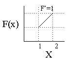
To illustrate, suppose we need to determine dF/dx at x=1, and our current
estimate is that F(1) = 1 and that F(2) = 2. Most likely, we would
simply connect the points with a straight line, as illustrated on the left,
and estimate that dF/dx ~ 1. This is a First Order Forward approximation;
first order because it uses one grid point besides x=1, and
forward because the grid point used is in the positive x direction
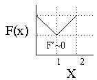
from x=1, the grid point for which we are making the estimate. However,
if we also know that F(0)=2, as shown on the right, we would probably guess
that there is a minimum at or near x=1, and thus estimate that dF/dx=0.
This is a Second Order Centered approximation; it uses two grid
points that are centered about x=1.
These examples are simply meant to illustrate the principles.
There isn't actually any "guessing" involved in Finite Difference methods;
equations derived from Taylor series expansions are used to compute the
best estimate of first and
second derivatives from a given set of grid points.
Selection of a Finite Difference Method
In general, it is best to use the Centered Finite Difference
method for systems in which convective flow and diffusion occur simultaneously.
For systems in which there is only convective flow, or in which diffusion
is also present but has a comparatively small effect, it is generally better
to use either the Forward or Backward Finite Difference method.
Use the one that runs opposite to the direction of the flow. In other
words, if the convective flow runs from z=0 to z=1, use the Backward
solution method for the z coordinate, and if the convective flow runs
from z=1 to z=0, use the Forward solution method.
The following Orders of Approximation are available:
Centered Finite Difference - 2, 4 or 6
Forward Finite Difference - 1 or 2
Backward Finite Difference - 1 or 2
Upwind-Biased Finite Difference - 2
Higher order approximations are viable in theory but are not currently
implemented in gPROMS.
Orthogonal Collocation on Finite Elements
An orthogonal collocation method uses a weighted combination of orthogonal
polynomials to approximate a solution. When this solution method
is selected, Order of Approximation refers to the order of the polynomials.
The solution method requires that the system equations are satisfied exactly
at a set of points called collocation points, which are the roots of one
of the polynomials. The number of collocation points is one greater
than the order of approximation, and the maximum and minimum of the domain
are two of the collocation points. The gPROMS solver outputs results
at these collocation points. Thus, if a third-order orthogonal collocation
is used as the solution method for the r-dimension of a cylindrical reactor
with 1 m radius, results will be generated at four values of r, including
r=0 and r=1 m.
One can also divide the domain of the problem into elements, and
apply a separate collocation to each. Continuing with the example
of a 1 m radius reactor, if one used 3 as the Order of Approximation
and 2 as the Number of Elements, then one order three collocation
would be applied to the range 0<r<0.5 and a second collocation would
be applied to the range 0.5<r<1.0.
The order of apprxomiation must be 3, 4 or 5.
This solution method is commonly used in reaction engineering.