Laboratory Project 2: Spatial and
Spectral
Filtering
Due Monday, Oct 19
This laboratory has three parts. In parts 1 and 2, you will experiment
with the characteristics of the Fourier transform (both continuous and
discrete) of a digital image. In part 3, you will develop both spatial
domain and spectral domain filters for image enhancement.
Part 1: Continuous Fourier Transform and Discrete
Fourier Transform of Images
Objective
The objective of this part is to model a simple image template both as
a continuous-space function and as a discrete-space function and
analytically determine its properties in the spatial and spatial
frequency domains.
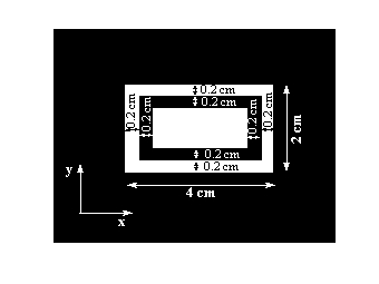
Figure 1: Image for Part 1.
Consider the image shown in Figure 1. DO NOT download
this
image! You are required to model it!
Model the image as a continuous-space 2-D function; and
plot.
Obtain, analytically, the Fourier transform of
the continuous-space image; and plot.
Based on your observations of the spatial frequency
components of the image; determine the maximum sampling interval
(delta_x = delta_y) / minimum sampling spatial frequency, that will
allow reconstruction of the original continuous-space 2-D
function / image.
Attempt to reconstruct the original continuous-space
function from its samples, either by:
Convolving the spatial domain samples with the appropriate
Sinc function (difficult), or
Windowing the continuous Fourier transform and taking the
inverse discrete Fourier transform (easier).
Compare with the original discrete-space sequence. Comment on your
results.
What is the maximum sampling interval / minimum sampling
frequency that will allow reconstruction of the the discrete-space
image from its Discrete Fourier Transform , that
adequately represents the original continuous-space image?
Part 2: Using the DFT to compute Spectral Components
Consider a 2-D function f(x,y) = sin(2*p*fx*x)
+ sin(2*p*fy*y) where fx and
fy are the spatial frequencies along the x- and
y-directions respectively. A digital image is generated by computing
this 2-D function over a spatial range 0 <= x <= S; 0 <=y
<=S, such that the range is divided into N equal points along both
the x- and y-directions.
Generate a sample image by choosing S = 1 cm, N = 128, fx =
30 per and fy = 50 per cm.
Compute the 2-D DFT of this image. Generate a surface-plot (>>
surf) of its amplitude spectum with the axes correctly indicating
the spatial frequencies.
Obtain an image of the amplitude spectrum.
Vary the parameters S, N, fx , and fy.
Comment on your results.
HINT: Use the 1-D DFT demo function shown at
http://engineering.rowan.edu/~shreek/spring07/ecomms/demos/dft.m
as a starting point.
Part 3: Spatial and Spectral Filtering
Objective
The objective of this part is to study the effects of low-pass and
high-pass filtering an image, using spatial domain and
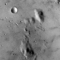
spatial-frequency domain techniques. Download the image of the Moon's
surface shown in Figure 2 obtained by one of the Ranger
Missions.
Figure 2: Moon image for Part 3.
Generate a 3 x 3 spatial averaging filter and perform a
neighborhood averaging over the original Moon image. Plot and observe
the Fourier spectrum of the averaged image; compare with the Fourier
spectrum of the original image.
Comment on your results.
Corrupt the original Moon image with a zero-mean Gaussian
noise, so that the SNR of the noisy image is 5 dB. Attempt to minimize
noise effects by using appropriate filters in
spatial domain, and
spectral domain.
Indicate the cut-off frequency of the spectral domain filter. Comment
on your results.
Corrupt the original Moon image with impulse (Salt and
Pepper) noise of density 0.01. Attempt to minimize noise effects by
using an appropriate spatial domain filter. Comment on your results.
Attempt to generate an image that contains only the edges
of the lunar craters, by high-pass filtering the original Moon image.
Do this using filters in both
spatial, and
spectral domains.
Is this possible? What cut-off frequency does the best job? Comment on
your results.
NOTE: For all results obtained using spectral domain filters,
you must provide images of