Digital Image Processing

Course Nos. ECE.09.452/ECE.09.552
Fall 2009 Laboratory Project 3: Degradation Models and Digital Image Restoration

Due Monday, Nov 23

Objective

The objective of this project is to study the effects of image degradations (in particular, blurring) and implement appropriate restoration techniques. This project has three parts. In Part 1, you will implement degradation and restoration techniques on a simulated image. In Part 2, you will attempt to replicate the degradation and restoration models illustrated in the textbook. In Part 3, you will attempt to restore a degraded image, given some information about the nature of the degradation and/or the original image characteristics.

Note: Display all images using a 256 gray-level map.

Part 1

In this part, you will investigate blurring and restoration techniques using a simple simulated image.

Generate a 12x12 discrete (space and intensity) model, f(x,y), of the image shown in the accompanying figure.

Figure 1: 12 x 12 discrete image model.

DO NOT download this image! You are required to model it!

Generate two sets of point spread functions (PSFs), h(x,y), one for simulating atmospheric turbulence and the other for simulating camera misfocus. These functions are shown below; the values of the scaling factors and the ranges of the blur-factors you are required to use in this project are indicated.

Figure 2(a): PSF for simulating atmospheric turbulence.

Figure 2(b): PSF for simulating camera misfocus.

For each of the PSFs in item 2, generate degraded images g(x,y) = f(x,y) * h(x,y), by convolving with the appropriate PSF. Do NOT add noise.

Using an inverse filtering technique, attempt to restore the degraded images, g(x,y). Calculate, for each case, the peak least squares error (PLSE). Tabulate your results.

Part 2

In this part, you will replicate the blurring and restoration techniques illustrated in the textbook on pages 260-265.

Part 2 (a): Atmospheric turbulence model and restoration using inverse and Wiener filters

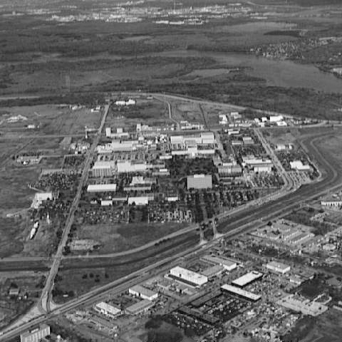
Download the aerial photography image shown in Figure 3 (same as Figure 5.25(a) in the textbook). Degrade the image to produce the severe, mild and low atmospheric turbulence shown in Figures 5.25 (b) through (d) of the textbook, using the model given by Equation 5.6-3.

Figure 3: Aerial photography image (480 x 480 pixels) shown in Figure 5.25(a) in Gonzalez & Woods.
(LEFT CLICK on image to get original)

Attempt to restore the degraded images using inverse filters - both full and radially limited. Use a Butterworth model for the cut-off in order to minimize spatial ringing. Figure 5.27 in the textbook illustrates typical results.
Attempt to restore the degraded images using Wiener filters. Figure 5.28 in the textbook illustrates typical results.

Part 2 (b): Planar motion model and restoration using inverse and Wiener filters

Download the textbook cover image shown in Figure 4 (same as Figure 5.26(a) in the textbook). Using the model shown in Equation 5.6-11 of the textbook, degrade the original image to the produce a set of 1-D and 2-D planar motion blurred images. Use the same parameters as given in the textbook (a = b = 0.1 and T = 1).
Also generate another set of images that include the effects of additive Gaussian noise (zero mean, variance of 650 pixels).

Figure 4: Textbook cover image (688 x 688 pixels) shown in Figure 5.26(a) in Gonzalez & Woods.
(LEFTCLICK on image to get original)

Attempt to restore the degraded images using inverse filters - both full and radially limited. Use a Butterworth model for the cut-off in order to minimize spatial ringing.
Attempt to restore the degraded images using Wiener filters. Figure 5.29 in the textbook illustrates typical results.

Part 3

In this part, you are presented with an actual image restoration problem for which you will make hypotheses, discuss and implement solution techniques.

Part 3 (a): Volumetric rendition of a human heart (Problem 5.20 in Gonzalez & Woods)

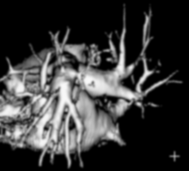
The image shown in Figure 5 is a blurred, 2-D projection of the volumetric rendition of a heart. It is known that each of the cross-hairs on the right, bottom part of the image was 3 pixels wide, 30 pixels long, and had gray level values of 255 before blurring.

Figure 5: Volumetric rendition of a human heart (623 x 563 pixels) shown in Problem 5.20 in Gonzalez & Woods.
(LEFTCLICK on image to get original)

Given this information, using a step-by-step procedure, determine the blurring function H(u,v).
Implement appropriate digital image restoration techniques on this blurred image.

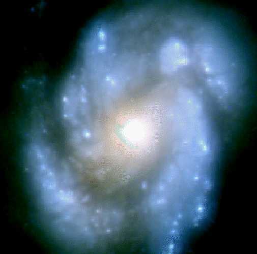
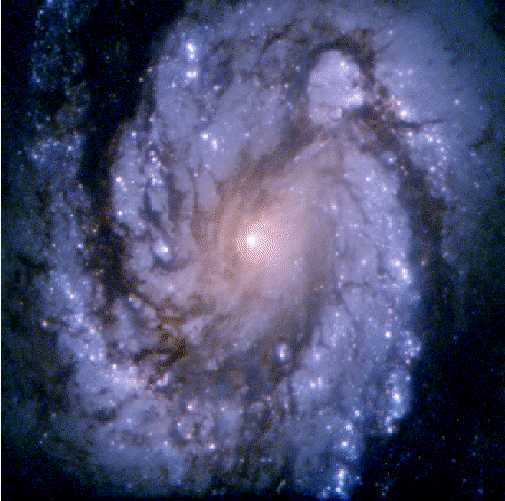
Part 3 (b): Spherical aberration in the Hubble Space Telescope prior to servicing

The first picture shown in Figure 6 below is that of the Spiral Galaxy M100, (in the constellation Coma Berenices), that was obtained by the Hubble Space Telescope in November 1993.

This picture is degraded (blurred), in a large part, to the effects of "spherical aberration" in the Hubble's primary mirror. Spherical aberration occurs when a spherical lens or mirror is improperly ground. Light rays near the edges of the lens/mirror are more strongly refracted/reflected and come to a focus nearer the lens/mirror than the rays closer to the axis.

Subsequently, a NASA space shuttle mission installed corrective optics to compensate for the Hubble's blurred vision. The result of this effort can be seen in the second figure, which shows the same M100 galaxy, obtained using the modified telecope. This image is one of the first post-servicing images.

Could we have obtained similar results using the image restoration techniques that were discussed in the class? What would be the effect of using inverse/Wiener filtering techniques, assuming PSFs of the forms used in parts 1 and 2 of this project? Demonstrate with examples.

Figure 6: Pre- and post- servicing Hubble telescope images of the M100 Spiral Galaxy.

Your report should be in the usual format.

Instructor

Schedule

Textbook

Tutorials/Demos

Grading

Homepage