FLUID MECHANICS 1 0901.341
Fall 1998
Chapter Review Guide for Fluid Mechanics, by Franzini et al. You can
use this page to test your understanding of each chapter. The focus is
identifying important equations and major concepts. However, don't use
this as an excuse for not reading the book! If you find any mistakes (typos,
etc.), let Dr. E. know as soon as possible!!
Back to Fluid Mechanics' home page
Table of Contents
Back to Table of Contents
Chapter 1
Approach to problem solving
Systems of units (BG and SI)
Dimensions (F, M, L, T)
Back to Table of Contents
Chapter 2
Concepts
Ideal fluid
Real fluid
Surface tension and capillarity
Vapor pressure
Variables
Density, r
Specific weight, g
Specific volume, u
Bulk modulus (also know as volume modulus), Eu
Specific gravity, s
viscosity (absolute and kinematic), m and
n
surface tension, s
wetting angle, q
Relationships
g = rg
u = 1 / r
Eu = -u
dp/du
Du / u y
- DP / Eu
s = r/rref
= g/gref
(where the reference substance is often water)
pu = RT
t= F/A = m U/Y
= m du/dy
n = m / r
h = (2s cos q)/
gr
Back to Table of Contents
Chapter 3
Concepts
Pressure at a point in a fluid is the same in all directions
Pressure varies as a function of depth and specific weight in fluids
Barometer
Pressure measurement
Bourdon gage, Pressure Transducer, Piezometer Column, Simple
and Differential Manometer
Forces and locations of forces on submerged plane and curved areas
Buoyancy and Stability
Fluid masses subjected to acceleration
Variables
Pressure head, h
Atmospheric, absolute and gage pressures, patm, pabs
and pgage
Centroid of area, hc, yc
Centroid of Pressure, hp, yp
Moment of Inertia (about an arbitrary axis and about a centroidal axis),
IO and Ic
Weight Force, W
Buoyancy force, FB
System subscript, S
Control volume subscript, CV
Relationships
DP/dz = - g
p = gh
h = p / g
pabs = patm + pgage
Be able to derive pressure relationships for piezometers and manometers
F = xp dA = ghcA
yp = IO / ycA = yc + IC
/ ycA
W = specific weight of object times its volume
FB = specific weight of water times volume of water displaced
by object
W = FB (for an object that is not rising
or falling in a fluid)
Back to Table of Contents
Chapter 4
Concepts
Ideal vs. real
Incompressible vs. compressible
Steady
Uniform
Laminar
Turbulent
Path line
Streamline
Flowrate (volume, mass, weight)
Mean velocity
System (S) and control volume (CV)
Continuity
Flow net, streamlines and equipotential lines
Velocity and acceleration in steady flow
Velocity and acceleration in unsteady flow
Variables
Volumetric flowrate, Q
Mass flowrate, m with dot on top (I'll just use m' here)
Weight flowrate, G
Velocity, V
Acceleration, a
Steady flow subscript, st
Bolding indicates a vector
Relationships
Q = VA
V = Q / A
m' = rQ (for constant
density flow)
G = gQ (for constant density
flow)
System - Control Volume Equation:
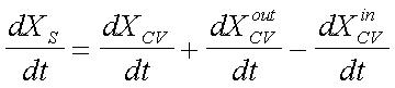
In words: change of X in the moving system equals change of
X within the control volume plus the flow of X out of the control volume
minus flow of X into the control volume.
A1V1 = A2V2 (incompressible
flow, steady flow)
r1A1V1
= r2A2V2 (steady
flow)
g1A1V1
= g2A2V2 (constant
gravity, steady flow)
ast = V cV/cs
(steady flow, s is direction tangent to streamline)
a = V CV/Cs
+ CV/ct
(unsteady flow, s is direction tangent to streamline)
Back to Table of Contents
Chapter 5
Concepts
Energy (kinetic, potential, pressure, internal,...)
General energy equation
Head (pressure, elevation, velocity, total, piezometric, static,...)
Power
Efficiency
Cavitation
Energy grade line
Hydraulic grade line
Head loss
Variables
a = Kinetic energy correction factor
I = internal energy per unit weight of fluid
p/g = flow work, pressure acting on flow
hM = shaft work, put into fluid by machine per unit weight
of fluid
QH = energy put into fluid by external heat source per unit
weight of fluid
hl = head loss
Relationships
Energy = Force time distance
Energy/unit weight has units of length
General energy equation (5.8):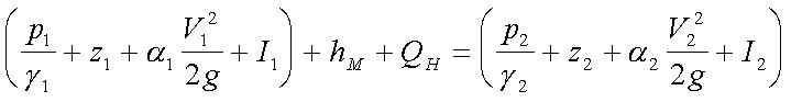
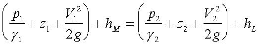
Bernoulli's equation (5.13):
hl = (I2 - I1) - QH
Power = hgQ = energy per time
Efficiency = power output / power input
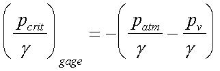
Cavitation (5.36):
Back to Table of Contents
Chapter 6
Concepts
Impulse-momentum principle
Navier Stokes equations
Force exerted on pressure conduits
Force exerted on stationary and moving vanes or blades
Absolute and relative velocities
Jets and Jet Propulsion
Pumps and Turbines, water
Head equivalent of hM
Reaction and rotating jets
Fans and Propellers, gases
Variables
Q' = rate of fluid striking a moving body, function of relative
velocities between water and body
V = absolute velocity of water
u = relative velocity of water (to some
moving body)
u = absolute velocity of moving body
Relationships
nF =
d(mV)s / dt
NF = rQ
(DV), for steady flow and stationary bodies
NF = rQ'
(Du), for steady flow and a single moving
vane (only a portion of fluid momentum is transfered)
NF = rQ
(Du), for steady flow and a series of moving
vanes (all fluid momentum is transfered)
hM = (u1 V1 COs a1
- u2 V2 COs a2)
/ g
Back to Table of Contents
Chapter 7
Concepts
Simlitude and Similarity
Reynolds Number
Froude Number
Mach Number
Weber Number
Scale Ratios
Dimensional Analysis and the Pi Theorem
Variables
Subscripts: p = prototype, m = model
Scale ratio, Lr
Velocity ratio, Vr
Force ratio, Fr
Reynolds number, R
Froude Number, F
Mach Number, M
c = sonic velocity in medium in question
Weber Number, W
s = surface tension
Relationships
R = LVr/m
F = V (gL)-0.5
M = V / c
W = V (s/rL)-0.5
Back to Table of Contents
Chapter 8a (sections 1 - 16)
Concepts
Laminar and Turbulent Flow
Critical Reynolds number
Laminar Flow, R <
2000
Friction in circular conduits
Friction factor
Pipe Roughness (hydraulically smooth, transitionally rough, fully rough)
Moody Diagram
Pipe flow Problems (head-loss, discharge, and sizing problems)
Solution of pipe flow problems using the Moody Chart
Solution of pipe flow problems using explicit equations
Empirical equations for pipe flow
Variables
Reynolds number, R
Hydraulic radius, Rh
Cross-section area of flowing fluid, A
Wetted Perimeter, P
Friction factor, f
Equivalent height of roughness projections, e
relative roughness, e/D
Energy Gradient, S (= hL / L, where L = length
of pipe)
roughness coefficients, CHW and n
Relationships
Rh = A / P
hl = f (L/D) (V2/2g)
f = 64/R, for laminar flow in circular pipes
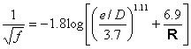 , for turbulent flow
Various derived and "fitted" equations, see especially pages 289-291.
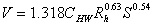 , BG units, formula is not unit-consistent,
limited applicability
, BG units, formula is not unit-consistent,
limited applicability
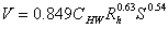 , SI units, formula is not unit-consistent,
limited applicability
, SI units, formula is not unit-consistent,
limited applicability
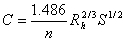 , BG units, formula is not unit-consistent,
limited applicability
, BG units, formula is not unit-consistent,
limited applicability
 , SI units, formula is not unit-consistent,
limited applicability
, SI units, formula is not unit-consistent,
limited applicability
Solutions
Type 1: solved directly. Type 2, and 3 problems:
solved iteratively using Moody's diagram, iteratively using equations,
or solved using equation solvers, see pages 294-302.
Empirical equations, see page 304-305.
Back to Table of Contents
Chapter 8b (sections 17 - 28)
Concepts
Minor Losses
When to include minor losses
When a fitting creates a major loss (such as a valve that is
almost closed)
For short pipe lengths (a good rule of thumb is to include minor losses
if the pipe length is < 1000 D)
Solution of various pipe problems
Variables
loss coefficient, k
equivalent length, L/D or N (multiply by pipe diameter, D, to estimate
equivalent length of straight pipe that would give same head loss as source
of minor loss)
Relationships, minor losses
Entrances: h'e = ke
V2/2g, where ke ranges ~0 to ~ 0.8, see
page 309.
Submerged discharges: h'd = V2/2g,
see page 310.
Contractions: h'c = kc
V2/2g, where kc is a function of D2/D1,
where D2 = diameter after contraction, D1
= diameter before contraction, kc ranges from 0 to
0.5, see page 312.
Expansions, sudden: h'x = (V1
- V2)2/2g, where V2
= velocity after contraction, V1 = velocity before
expansion
Expansions, gradual: h' = k' (V1
- V2)2/2g, where V2
= velocity after contraction, V1 = velocity before
expansion, and k' is a function of cone angle, see page 316.
Pipe fittings: h = k V2/2g, where k depends on the
fitting, see page 317. Alternatively, one can use the equivalent
length concept (L/D from Table 8.3 times the pipe diameter). Add
the equivalent length of the fitting to the pipe length. This ensures
that the head loss caused by the fitting is taken into account, but as
pipe friction.
Bends: hb = kb
V2/2g, where kb is a function of relative
roughness and the ratio of the bend radius to the pipe diameter, see page
320.
Solutions, of specific types of pipe problems
Single-pipe flow with minor losses: Total head
loss is sum of pipe friction loss and minor loss, see page 321.
Pipeline with pump or turbine: Total head provided by
a pump or supplied to a turbine is a function of energy (change in elevation
and velocity, usually) and the pipe friction and minor losses, see page
327. Minor losses are often ignored.
Branching pipes: Need to use continuity and energy equations,
see page 331. Minor losses and even velocity heads are often ignored.
Pipes in series: Continuity shows that the flow through
each pipe is the same, the total head loss is the sum of the head loss
in each pipe. See page 338.
Pipes in parallel: Continuity shows that the
flow through the system is the sum of the flows in the individual pipes.
The head loss to get from point 1 to point 2, through any of the pipes,
is the same, therefore the head loss of each pipe is the same, see page
341.
Back to Table of Contents
Back to Fluid Mechanics' home page
qwertyuiopasdfghjklzxcvbnmQWERTYUIOPASDFGHJKLZXCVBNM
qwertyuiopasdfghjklzxcvbnmQWERTYUIOPASDFGHJKLZXCVBNM