| 
Laboratory
Project 1 - Waveform Synthesis and Spectral Analysis
Objectives
Laboratory project 1 contains 4 parts. In Part 1, you will:
* Generate arbitrary waveforms with specified SNR's using software;
* Synthesize this waveform using an arbitrary waveform generator.
In Part 2, you will study the differences between the Continuous
Fourier Transform (CFT) and the Discrete Fourier Transform (DFT)
(this is homework!).
In Part 3, you will synthesize AM and FM bandpass signals and analyze
their spectra.
In Part 4, you will capture and analyze the spectrum of an electrocardiogram
(ECG/EKG) signal.
Equipment and Software
* HP 33120A Function/Arbitrary Waveform Generator
* Agilent Infinium Oscilloscope
* BNC "TEE" connector
* Powered speakers with 3.5mm stereo connector
* Wireless breadboard
* Convert-o-box (supplied with lab kit)
* Clinimark Pinstyle ECG Electrodes and leads
* Antiseptic prep pads
* Human with beating heart (or, if absent, a Lionheart 3 cardio-simulator)
* 9VDC battery
* 50ohm BNC Cable
* ECG module
* MATLAB (with Instrument Control Toolbox)
* MATLAB Connectivity Functions: >>writefunc(.),
>>scopedat(.)
Click
here for instrument connectivity guide and Matlab function downloads
required
Instrument Connectivity
In this, and future labs, you will be required to send and gather
data to various instruments at the station. To do this, you will
need an active connection with the instruments by opening and refreshing
the instruments in Agilent IO Libraries. Click Start>All Programs>Agilent
IO Libraries Suite>Agilent Connection Expert. When the software
is open, click the refresh button until the instrument icons are
green. Obvioulsy the instruments will need to be powered on and
past initialization before they are seen by Connection Expert.
You will also need the board index (the 'number' of the interface
card), and the GPIB address of the instrument. To find the board
index, open the tmtool link under Matlab>Start>Toolboxes>Instrument
Control>Test and Measurement Tool (tmtool) OR type >>tmtool
in the Matlab command window. Expand the Hardware and then the GPIB
tab on the lefthand pane. The board index should be either 7 or
8. You will see that boards that have instruments connected to them
will be expandable. The GPIB addresses are consistent across all
instruments in the Mixed Signals Laboratory:
Oscilloscope: 7
HP8648A: 9
HP33120A (Upper): 10
HP33120A (Lower): 11
HP34970A: 12
Keithley 2000/2100: 16
HP/Agilent E3631A: 5
->
Please read the connectivity guide for full details
Part 1: Digital synthesis of arbitrary waveforms
with specified SNR
Background
Procedure
* Synthesize a 1 second A-Sharp sinusoidal tone (466.16 Hz)
sampled at 8 kHz.
* Plot this waveform; observe. Save this waveform to a .wav
sound file, play and listen. (You can listen using the sound command
in Matlab)
* Send the data to the HP33120 Arb. Function Generator using
the >>writefunc(.) function in Matlab. NOTE: the
HP33120A function generators and the >>writefunc(.)
function can only handle <= 16,000 data points. You can
check the length of your data vector by running the >>size(data)
command. Please read help file: >>help writefunc.
It must also be noted that the data, by default, is stored in
the workspace. Any >>clear all or variable overwrite
commands will remove the data! If you would like to save the data
to the HDD, use Matlab's >>save(.) function. Also
mind frequency scaling which can occur if improper considerations
are made with regard to time vector length and signal generator
frequency setting.
- Send one second of the sinusoid to the function generator
and confirm via. data capture. In the >>writefunc(.)
command, set FREQ to 1. This (coupled with the 1 second data
length) will ensure that the sinusoid's specified frequency
is maintained.
- If you wish to experiment: Note that for periodic
waveforms, all that is required for perfect synthesis
is one period of the signal. This means that ALL available memory
(16k) can be 'stuffed' into the minimal amount of time required
(i.e. one period), giving a much higher resolution signal. This
method requires alternate consideration for obtaining the proper
frequency, however! Experiment!
* Corrupt the signal (1 second of the A-sharp sinusoid) with
a Gaussian noise source to get an SNR of 10 dB. Observe, listen
and save waveform as before.
* Synthesize 1 second of the noisy waveform.
* Download the original and noisy signals to the HP33120A Arbitrary
Function Generator using the MATLAB connectivity function: >>writefunc(.)
. NOTE: Any amplitude sent to the function generator is normalized
over a +/- 1 range. Real amplitude output voltage is controlled
by the 'AMP' argument in the function. For noisy waveforms, outliers
will appear at the extremes. A practical range should be specified
so that the amplitude is correct. Any real amplitudes over 10Vpp
cannot be realized on the HP33120A Function Generator.
* Vary the frequency and amplitude. Observe waveform using the
oscilloscope.
* Repeat experiment with various SNRs.
* Experiment with other waveforms:
Example Matlab Code:
%ECOMMS
Lab Project 1 Example Spring 10
%S. Mandayam,
Rowan University
%This program generates a 1-second duration
%Asharp signal (466.16 Hz) with a specified SNR
%Specify
SNR
snr=10;
%Generate
Asharp signal
t=[0:1/8e3:1.0]';
s = 0.5*sin(2*pi*466.16*t);
sound(s);
wavwrite(s, 'asharp.wav');
save asharp.csv -ascii s;
%Compute
signal variance
var_s = cov(s);
%Calculate
required noise variance
var_noise=var_s/(10^(snr/10));
%Generate
noise
n=sqrt(var_noise)*randn(length(s),1);
sound(n);
%Add signal
to noise and generate message
m=s+n;
sound(m);
wavwrite(m,'asharp_noise.wav');
save asharp_noise.csv -ascii m;
Part 2: Comparison between CFT and DFT (FFT)
(Uses Matlab only - this is homework!)
Consider the signal shown in Figure 1:
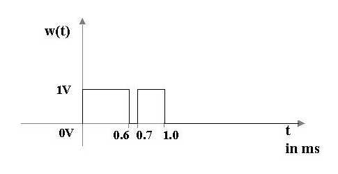
Figure 1: Time-domain signal
* Model the signal as a continuous-time function and plot.
* Obtain, analytically, the CFT of the signal, and plot.
* Based on your observations of the frequency components of the
signal, determine the maximum sampling period/minimum sampling
frequency that will allow reconstruction of the continuous-time
signal.
* Plot the DFT magnitude spectrum using Matlab's fft function.
* Attempt to reconstruct the original continuous-time function
from its samples, either by: Convolving the time domain samples
with appropriate Sinc function (difficult), or Windowing the Fourier
transform and taking the inverse Fourier transform (easier).
* Comment on your results. What is the maximum sampling period/minimum
sampling frequency that will allow reconstruction of the discrete-time
signal from its DFT, that adequately represents the original continuous-time
signal? Show plots of the discrete-time signals, the corresponding
DFTs and reconstructions, for sampling intervals at, above and
below this maximum allowed sampling period.
Part 3: Spectral Analysis of AM and FM
Signals
(Uses Matlab, Oscilloscope, Function Generator and Spectrum Analyzer/FFT
module)
* Synthesize a bandpass AM signal:

* Obtain and plot the spectral components of this signal using:
1. Matlab's fft function.
2. The spectrum analyzer/FFT module.
* Add noise to the RF signal, observe the signal in the time
and spectral domains.
* Experiment with various fm's, fc's
and SNRs.
* Synthesize a bandpass FM signal:

* Repeat earlier experiments.
Part 4: Spectral Analysis of ECG Signal
(Uses Matlab, Oscilloscope, ECG Electrodes and leads, Antiseptic
Prep Pads, 9VDC battery, 50ohm BNC cable, ECG module, and Spectrum
Analyzer/FFT Module)
NOTE: READ THIS FIRST!!!
This experiment must be conducted with the instructor present at
all times when you are obtaining the ECG readings. The procedure
that has been outlined below has been determined to be safe for
this laboratory. You must use an isolated power supply (9VDC Battery)
for powering the ECG module. This objective of this experiment is
compute the amplitude-frequency spectrum of real data - this experiment
does not represent a true medical study; reading an ECG effectively
takes considerable medical training. Therefore, do not be alarmed
if your data appears"different" from those of your partners.
Also, if you observe any allergic reactions when you attach the
electrodes (burning sensation, discomfort), remove them and rinse
the area with water. Finally, if, for any reason, you do not want
to participate in this experiment, obtain recorded ECG data from
your instructor.
* Electrocardiagram (ECG or EKG) measurements are used to monitor
the contraction of the cardiac muscles by measuring the propagation
of electrical depolarization and repolarization in the atria and
ventricles. The ECG is one of the many diagnostic tools for monitoring
the normality of cardiac activity in a patient. The references
provided below provide considerable additional information regarding
the ECG. Figure 2 shows the components of a typical ECG signal.
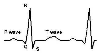
Figure 2: Components of a typical ECG signal
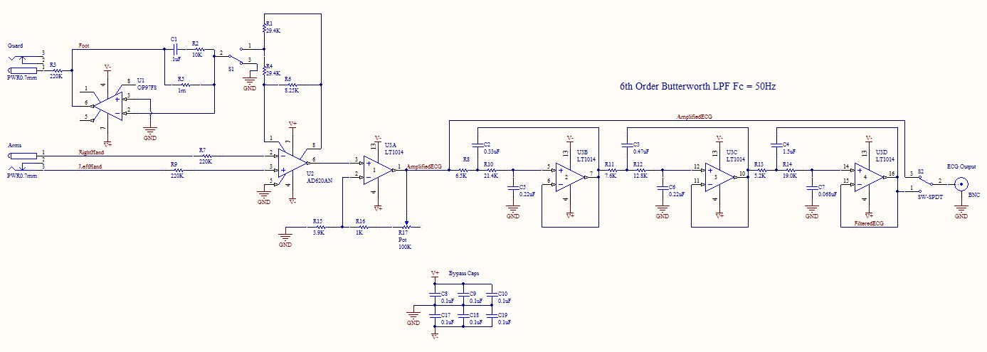
* The schematic of the ECG module is shown in Figure 3.
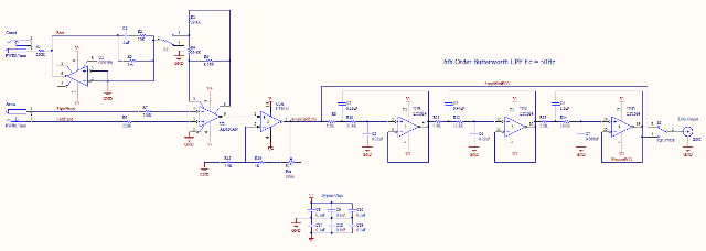
Figure 3: Schematic of ECG module. Click to enlarge
* This module includes many features including:
- 2 (arms) or 3 lead (arms + leg) electrode tests. NOTE: for
this lab, you will be doing a 2-lead experiment only (one electrode
pad on each wrist). Be sure the "Guard" switch is
in the OFF position and you use the correct electrode jack ("Arms").
- Adjustable gain (the "Gain" trimmer potentiometer
located in the center of the PCB)
- 6th order Butterworth LPF with cutoff set at 50Hz (switchable
on/off via the "LPF" switch)
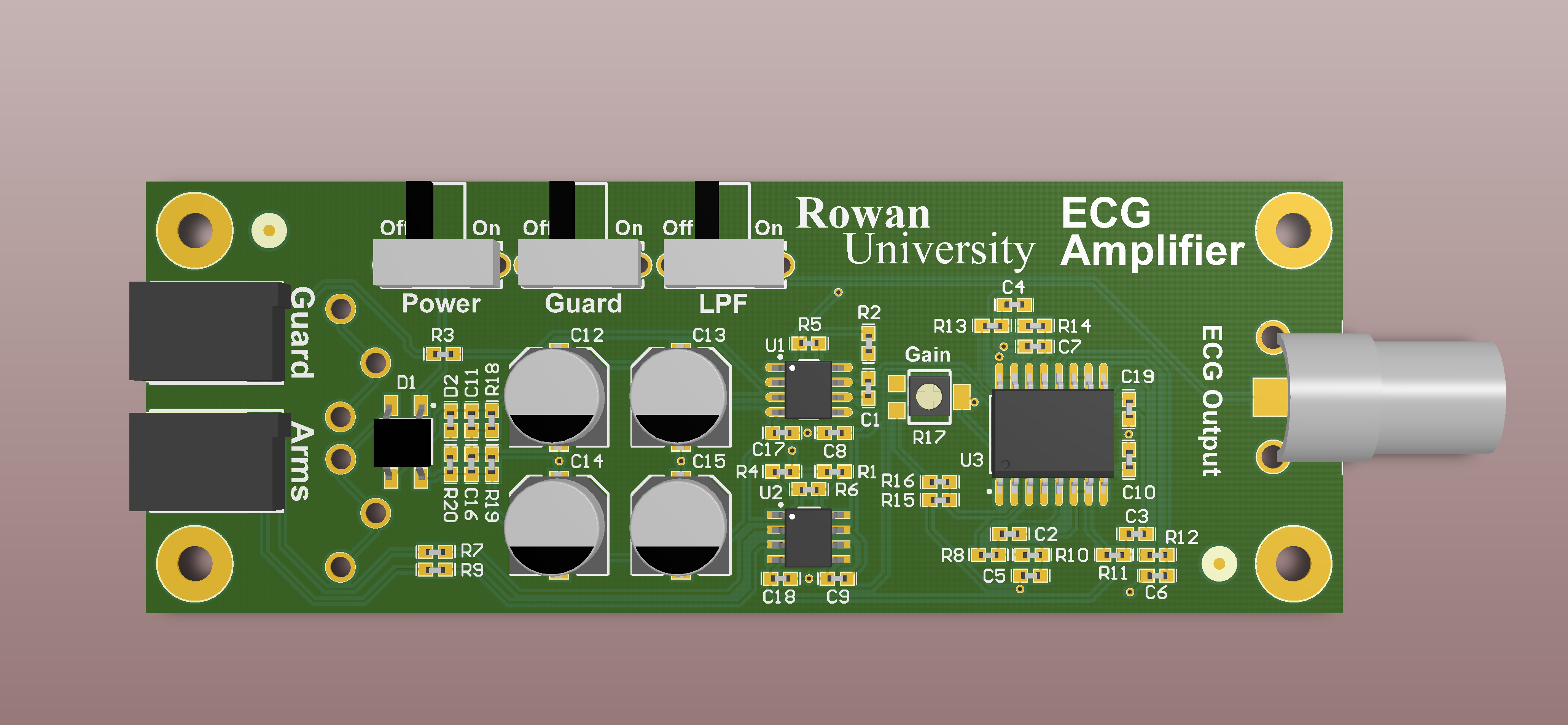
* The PCB layout of the ECG module is shown in Figure 4.
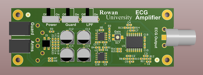
Figure 4: PCB layout showing locations of important components.
Click to enlarge
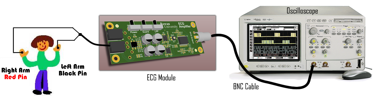
* The experimental set-up for taking ECG measurments with the
supplied ECG module is shown in Figure 5.
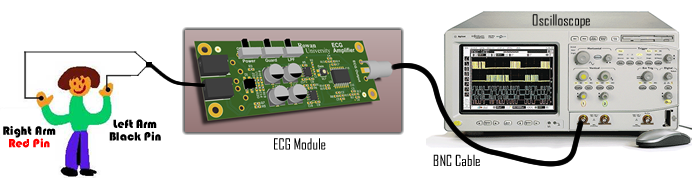
Figure 5: Experimental set-up for taking ECG measurements. Click
to enlarge
* Select one of your lab partners as the "patient"
for obtaining the ECG. Use the antiseptic prep pads and thoroughly
clean the wrist area where the electrodes will be attached. A
thorough cleaning is required to ensure a good contact of the
electrode with the skin - and a strong signal.
* Remove the electrodes from the release sheet and place each
electrode on the inside wrist of each arm. (This method of electrode
placement is known as Standard I Lead). Press firmly to ensure
adequate contact.
* Attach the electrode lead wire pin into the hole on the top
of the electrode. The other end of the lead wire is connected
to the "Arms" jack on the ECG module. Be sure the "Guard"
switch is in the "Off" position.
* Use a 50ohm BNC cable and connect the output terminal of the
ECG module to the oscilloscope.
* With the instructor present,
power on the ECG module by switching the POWER switch to the ON
position. Observe the ECG signal on the oscilloscope. To obtain
a strong signal, you may need help from your lab partner to press
the electrodes firmly to your arm. Be as still and quiet as possible;
any movement will induce noise and shift the ECG signal.
* Baseline scope settings should be 500ms/div to 1s/div. Most
scopes display a small arrow pointing to where the signal is located,
if it is off-screen. You may also wish to simply press the 'autoscale'
button, then adjust the time scale accordingly (most likely, the
autoscale will set the scope's focus on a much 'faster' part of
the waveform).
* The "Gain" potentiometer on the ECG may be rotated
clockwise with a trimmer screwdriver if additional amplification
is needed.
* Capture the waveform using the >>scopedat(.)
Matlab function, ensuring the 'patient' is as still as possible.
Also be certain the FILTER switch is OFF. You may observe a strong
60 Hz ripple - you can eliminate this by filtering the signal
using DSP techniques.
* Capture the ECG waveform again, but now with the LPF switch
in the ON position. This will enable the on-board analog LPF and
remove most of the 60Hz noise.
* Comment on the time and frequency components of the ECG signals.
Click
here for required lab project report format.
Click
here for suggestions for a good lab report.
References:
* HP 33120A Function Generator/Arbitrary Waveform Generator
User's Guide
* Appendix B (p. 650) in textbook
* Zsolt Papay, Technical University of Budapest (TUB),"Experiments
in Gaussian White-noise Generation," HP Test and Measurements
Educator's Corner, http://www.home.agilent.com/upload/cmc_upload/All/Exp65.pdf
* Chapter 2 in the texbook.
* Class Demo: Sampling
* Class Demo: Discrete
Fourier Transform
* Class Demo: Spectrum Analyzer
* L. A. Geddes and L. E. Baker, Principles of Applied Biomedical
Instrumentation, 2nd Edition, Wiley, 1975.
* Frank G. Yanowitz, MD, University of Utah School of Medicine,
The Alan E. Linday ECG Learning Center in Cyberspace, http://www-medlib.med.utah.edu/kw/ecg/ecg_outline/
|