| 
Laboratory
Project 2 - AM & DSB-SC Modulation and Detection
Objectives
This lab project consists of 2 parts. In Part 1, you will investigate
the performance of the simple envelope detector. In Part 2, you
will generate and detect AM and DSB-SC bandpass signals using the
LM1596/LM1496 Balanced Modulator-Demodulator.
This lab introduces the brand new Rowan University Modular Backplane
system. This system will be outlined below.
In both parts, you will test the system with single-tone AM (with
and without added Gaussian noise) and multi-tone AM signals (without
added noise).
Equipment and Software
* HP 33120A Function Generator/Arbitrary Waveform Generator
* Agilent Infiniium Oscilloscope
* Modular Backplane
* Envelope Detector Module
* Audio Preamplifier Module
* AM Modulator Module
* 5kHz LPF Module
* Standard AM Demodulator Module
* DSB-SC AM Demodulator Module
* Assorted Resistors and Capacitors (based on design of filter).
* PC speakers
* Breakout Board
* 3.5mm Stereo Cable
* Audio Player Software on PC
* CD/mp3 with your favorite music!
* MATLAB (with Instrument Control Toolbox)
* MATLAB Connectivity Functions: >>writefunc(.),
>>scopedat(.)
Click
here for instrument connectivity guide and Matlab function downloads
Instrument Connectivity
In this, and future labs, you will be required to send and gather
data to various instruments at the station. To do this, you will
need an active connection with the instruments by opening and refreshing
the instruments in Agilent IO Libraries. Click Start>All Programs>Agilent
IO Libraries Suite>Agilent Connection Expert. When the software
is open, click the refresh button until the instrument icons are
green. Obvioulsy the instruments will need to be powered on and
past initialization before they are seen by Connection Expert.
You will also need the board index (the 'number' of the interface
card), and the GPIB address of the instrument. To find the board
index, open the tmtool link under Matlab>Start>Toolboxes>Instrument
Control>Test and Measurement Tool (tmtool) OR type >>tmtool
in the Matlab command window. Expand the Hardware and then the GPIB
tab on the lefthand pane. The board index should be either 7 or
8. You will see that boards that have instruments connected to them
will be expandable. The GPIB addresses are consistent across all
instruments in the Mixed Signals Laboratory:
Oscilloscope: 7
HP8648A: 9
HP33120A (Upper): 10
HP33120A (Lower): 11
HP34970A: 12
Keithley 2000/2100: 16
HP/Agilent E3631A: 5
->
Please read the connectivity guide for full details
Modular System Overview
Lab 2 introduces the new, fully modular backplane system (MBS),
Figure 1, which you will use for the remaining labs in Ecomms. This
system saves you the tedious process of prototyping all of the circuits
required to complete the labs.
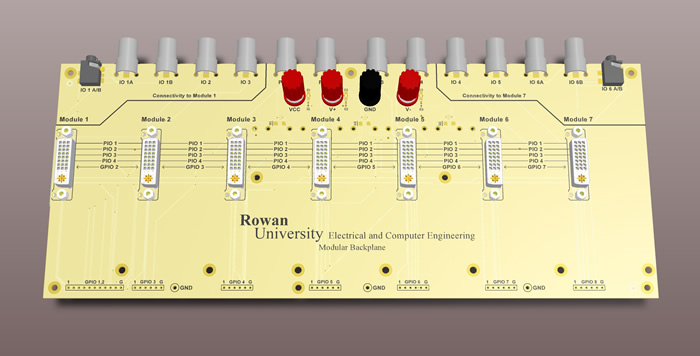
Figure 1. Modular Backplane. Click
to enlarge
This system is comprised of a modular backplane, which supplies
power, baseband and RF connectivity, and GPIO to the inserted modules.
The backplane has locations for up to 7 modules, which are installed
in the DVI connectors on the board. The first (module location 1)
and last (module location 7) modules are important and have special
connectivity to the screened off sections (IO1, 2, 3 and IO 4, 5,
6). Generally, you should always put your first (input) and last
(output) modules in the Module 1 and Module 7 positions, respectively.
It is important to note that the backplane is designed with both
parallel and serial connectivity between the modules. This means
that some IO are connected to ALL modules and some are only transferred
into a module. Parallel IO (PIO Ports 1 thru 4) are selected by
the layout of the specific modules so you must use the appropriate
PIO specified by the module you are using (connections are marked
on the module PCBs). The serial connectivity is utilized for inputs
that are fed to a processing block on a module, processed, then
output to another pin. Serial IO is only user-accessible via. the
GPIO headers.
The GPIO headers at the bottom of the backplane tap into all tranferred
IO between each module slot. This allows direct access of any signal,
if needed.
The modules for this kit will vary depending on the application.
It is up to you to decide the proper locations and signal path for
your application. The backplane has no physical lockout for placing
certain modules in certain locations to retain full functionality,
so you must be very careful in laying out your system. Some modules
include: Audio Preamplifier, 5nkHz Filter, Envelope Detector, AM
Mod/Demod, FM Tx/Rx, etc...
If you need to get from one end of the board to the other and your
application calls for less modules than slots, then you can use
a jumper. This jumper simply transfers any serial connectivity between
slots to the next, adjacent slot. You are supplied with 4 jumpers
in your kit.
Most modules have test points located at the bottom edge of the
PCB. These points are to be used with the hook of a scope probe.
Grounds are convieniently located on the backplane. Test point maps
will be specified in the lab pages.
The kit is also supplied with a breakout board, which can be used
as a general purpose adapter to convert, for example, a BNC type
connection to 3.5mm stereo.
All components of the MSB are housed in a custom case. When finished,
mount the backplane with (AT LEAST!) 2 modules installed, place
on its stand, and close the lid. This applies the correct amount
of pressure to the plane and keeps it secure during transport. Ensure
all modules are placed in their appropriate cutouts and any cables
are coiled and placed neatly in the circular cutout. Do not leave
any components loose!
Part 1
* The circuit for the passive envelope detector is shown in Figure
2. The design equation for the first-order low-pass filter made
up by C1 and R1 is:

* C2 is a coupling capacitor, chosen such that C2 >> C1.
Note that this capacitor also forms a filter with the load impedance
so you may wish to discover what rolloff is created here. As initial
design parameters, choose a cut-off frequency of 5 kHz. (As part
of the theory section in your report, you are expected to derive
this design equation).
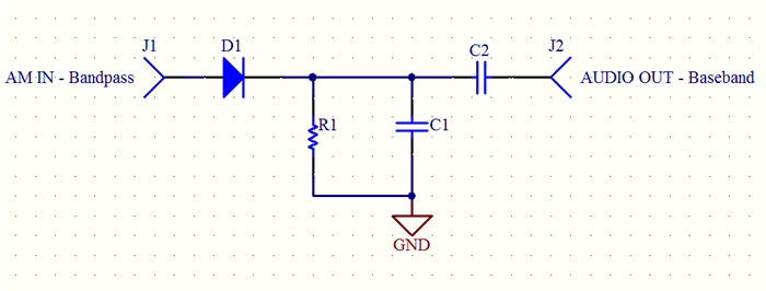
Figure 2. Passive Envelope Detector Circuit
* The envelope detector has been fabricated as
a module, which is to be plugged-in to the modular backplane.
This module has provisions for inserting the selected C1 and R1
components. Locations of these components are shown in Figure
3 below. NOTE: There is a RefDes on the board
'C1' in black silkscreen. This is NOT the C1 as above. The actual
RefDes is C5 on the board. You will plug in the resistor and capacitor
leads into the sockets in these positions.
Click here for
the full schematic of the envelope detector module (includes circuit
locations of test points).
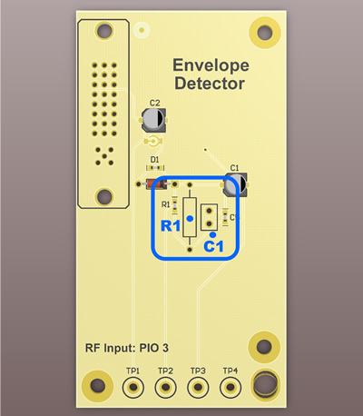
Figure 3. PCB locations for C1 and R1 on the Envelope Detector
Module. Click to enlarge
Single-Tone AM Detection: No added Gaussian
Noise
* Using the HP/Agilent Arb. Function Generator, generate an
AM wave with carrier frequency of 600 kHz (in the AM band) and
modulation frequency 1 kHz (single tone). Feed this signal to
the input of the envelope detector.
- Vary the modulation depth from 10% to 120%.
- For each modulation depth, observe and digitally capture the
input and output waveforms using the scopedat.m MATLAB function.
- Perform a spectral analysis of the input and output waveforms.
Observe the spectral components due to ripple and harmonic distortion.
You may want to view the signal's spectrum using the oscilloscope
FFT-Magnitude function before pulling data to MATLAB. To use
the scope's FFT properly, you will likely need to manually set
the frequency span and center. As with any spectrum analysis,
you should have some idea what frequencies you are looking for
(choose these settings accordingly).
- Listen to the output signal using the PC speakers. Note that
the PC speakers and audio output of most consumer electronics
is in stereo. This means each right/left channel has a distinct
audio signal. In this lab, using only one detector, you will
only be able to listen to one channel of audio and will effectively
be 'mono.'
- Compare the signal with the pure tone of the same frequency.
* Set the modulation index to an optimal value (max value for
minimum distortion) and vary the modulating signal frequency to
determine the 3-dB bandwidth of the detector (value at which the
output signal falls to 0.707 of its maximum value).
* Experiment by varying the carrier frequency and/or cut-off
frequency of the LPF.
Multi-Tone AM Detection: No added Gaussian
Noise
Figure 4 shows the overall block diagram for this part of the
lab project.
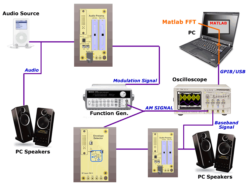
Figure 4: Multi-tone AM generation and detection.
* Obtain a multi-tone baseband signal by playing a CD on your
PC, an mp3 on your favorite portable audio device, or mp3 on your
PC and tapping into D/A converter output of the sound card (i.e.
the headphone jack).
* Feed this baseband signal into the external AM modulating source
input located on the back of the HP/Agilent 33120A Function Generator.
* Set the function generator to AM with EXTERNAL source. There
should be an 'EXT' string displayed on the front panel indicating
the AM modulator of the function generator will use the external
port as the modulation source.
* Choose a suitable carrier frequency in the AM broadcast band
('medium wave' AM is most common for broadcast AM radio) and generate
an AM signal.
* Observe the modulated signal on the oscilloscope. Vary the
modulation depth by varying the gain of the operational amplifier.
* Apply the multi-tone AM signal to the input of the envelope
detector. For each modulation depth:
- Observe, calculate the modulation depth and digitally capture
the input and output waveforms.
- Perform a spectral analysis of the input and output waveforms.
Single-Tone AM Detection: With added Gaussian
Noise
* Repeat the single-tone AM detection experiment by digitally
synthesizing single-tone AM signals with varying SNR in MATLAB
as you did in Lab 1. As always, pay special attention to sampling
and duration of your synthesized waveform and the frequency and
amplitude settings of the function generator. Figure 5 shows the
overall block diagram for this part of the lab project.
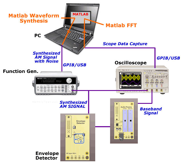
Figure 5: Block diagram of the approach for single-tone AM detection
with added Gaussian noise.
* At each stage, note your observations and conclusions.
Part 2
The obective for part 2 is to observe (in both the time and spectral
domains) & listen as audio progresses along a modulation-demodulation
system, both in the presence and absence of added Gaussian noise.
* Configure the system for standard AM as shown in Figure 6
below. As an initial test, determine the system response by feeding
two audio-frequency (<20kHz) tones to the input pins. The carrier
signal amplitude should be 300mVRMS or about 1Vpp. Observe the
waveforms on the oscilloscope and listen to the output using the
speakers. NOTE: if you want to hear the 'volume'
swell of the AM signal (which audibly demonstrates 'Amplitude
Modulation') be sure you choose an appropriate message frequency
(i.e. below ~10Hz). If it is too fast, it will simply sound like
another tone.
Full schematics for each module are provided below (this includes
circuit access for each test point):
AM Modulator
AM DSB-SC Modulator
AM Demodulator
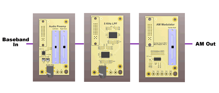
Figure 6: System configuration for standard AM modulation.
* Now increase the carrier signal frequency to the RF range
and observe the output waveforms.
* Now connect the AM DSB-SC modulator module in place of the
standard AM module. Vary the carrier null potentiometer to trim
the DSB-SC modulation. Observe the system response both in the
time and spectral domains (you need to perform a signal capture
followed by an FFT operation to do this). Confirm the carrier
null by viewing it in the frequency domain (use the scope's FFT-Magnitude
function).
* Experiment with various carrier and modulation frequency settings.
* Vary the modulation signal amplitude - calculate the corresponding
changes in modulation index. Determine the spectral response.
* Repeat the experiment by mixing in a multi-tone modulating
signal (generated as in Part 1).
* Now configure the system for AM demodulation as shown in figure
7. Test the circuit by feeding in an external modulation multi-tone
AM signal from the arb. Observe and listen to the audio output.
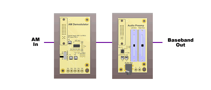
Figure 7: System configuration for AM demodulation.
* Test the product detector by feeding in digitally synthesized
single-tone AM and DSB-SC signals with varying SNR. When does
the modulator fail to detect the message signal? NOTE:
The MC1496 AM demodulator performs best when the carrier
frequency is above 100kHz.
* Link the modulator-demodulator circuits and observe signal
progression from input to output. Be sure to capture screenshots
to confirm the proper progression of the signal from baseband-to-baseband.
Required Reading
* Sections 4.11 - 4.13, 5.1 - 5.4 of textbook.
* User's Guides for HP 33120A Function Generator/Arbitrary Waveform
Generator, Agilent Infiniium Series Oscilloscopes
Click
here for required lab project report format.
Click
here for suggestions for a good lab report.
References:
* HP 33120A Function Generator/Arbitrary Waveform Generator
User's Guide
* Appendix B (p. 650) in textbook
* Zsolt Papay, Technical University of Budapest (TUB),"Experiments
in Gaussian White-noise Generation," HP Test and Measurements
Educator's Corner, http://www.home.agilent.com/upload/cmc_upload/All/Exp65.pdf
* Chapter 4, 5 in the texbook.
* Class Demo: Sampling
* Class Demo: Discrete
Fourier Transform
* Class Demo: Spectrum
Analyzer
* Class Demo: Amplitude
Modulation
* Class Demo: DSB-SC
|